Carpyncho RR-Lyrae V.1.0 Catalogs(cp_rr_v1)

This notebook give some insights about the data stored in all the features types catalogs.

# import the module and instance the client
import carpyncho
client = carpyncho.Carpyncho()

Now we download te Carpyncho RR-Lyrae V1 Catalog

df = client.get_catalog("others", "cpy_rr_v1")
df

others-cpy_rr_v1: 32.8kB [00:00, 1.80MB/s]

	id	tile	cnt	ra_k	dec_k	prob	tsample
6799063	33960000211620	b396	131	267.549917	-18.699892	0.852000	b206, b214, b216, b220, b228, b234, b247, b248...
7153972	33960000942530	b396	130	268.118017	-17.763556	0.849467	b206, b214, b216, b220, b228, b234, b247, b248...
6971905	33960000566886	b396	131	267.536346	-18.093889	0.837733	b206, b214, b216, b220, b228, b234, b247, b248...
6801853	33960000220135	b396	131	267.637892	-18.734767	0.837333	b206, b214, b216, b220, b228, b234, b247, b248...
6747151	33960000105195	b396	131	267.487762	-18.848939	0.828400	b206, b214, b216, b220, b228, b234, b247, b248...
...	...	...	...	...	...	...	...
6457949	33600000787886	b360	139	263.635417	-29.303825	0.462667	b206, b214, b216, b220, b228, b234, b247, b248...
6926060	33960000470380	b396	131	267.525504	-18.250553	0.462000	b206, b214, b216, b220, b228, b234, b247, b248...
6874859	33960000359818	b396	131	267.490592	-18.416206	0.460933	b206, b214, b216, b220, b228, b234, b247, b248...
682776	32200000656825	b220	123	274.725521	-34.229878	0.460933	b206, b214, b216, b228, b234, b247, b248, b261...
6617136	33600000965623	b360	204	263.473292	-28.911094	0.460533	b206, b214, b216, b220, b228, b234, b247, b248...

242 rows × 7 columns

The columns of this catalog are

print(list(df.columns))

['id', 'tile', 'cnt', 'ra_k', 'dec_k', 'prob', 'tsample']

Where

• id (ID): This is the unique identifier of every light curve. If you want to access all the points of the lightcurve of a source wiht any id, you can search for the same value of a bm_src_idin the lc, or id in the features catalog of the same tile indicated in the column tile.
• tile: The name of the tile where the candidate is located.
• cnt (Count): How many epochs has the lightcurve.
• ra_k: Right Ascension in band \(K_s\) of the source in the first epoch.
• dec_k: Declination in band \(K_s\) of the source in the first epoch.
• prob (Probability): The probability of this source to be a RR-Lyrae star [1].
• tsample (Tiles-Sample): Which tiles was used to create the ensemble select this source as a candidate [1].

[1] To more insights about this feature please chek our work

Not ready

Well lets play with a candidate

rr = df.iloc[0]
rr

id                                            33960000211620
tile                                                    b396
cnt                                                      131
ra_k                                              267.549917
dec_k                                             -18.699892
prob                                                   0.852
tsample    b206, b214, b216, b220, b228, b234, b247, b248...
Name: 6799063, dtype: object

We can check their mean of magnitudes to check if the source is not saturated or diffuse.

Now we know id from the tile b396 we can retrieve the entire collection of features and the light-curve

feats = client.get_catalog("b396", "features")
lc = client.get_catalog("b396", "lc")

# retrieve the features of the selected source
feats = feats[feats.id == rr.id]
lc = lc[lc.bm_src_id == rr.id]

b396-features: 303MB [02:10, 2.32MB/s]
b396-lc: 829MB [05:58, 2.32MB/s]

No we have the features

feats

	id	cnt	ra_k	dec_k	vs_type	vs_catalog	Amplitude	Autocor_length	Beyond1Std	Con	...	c89_jk_color	c89_m2	c89_m4	n09_c3	n09_hk_color	n09_jh_color	n09_jk_color	n09_m2	n09_m4	ppmb
144267	33960000211620	131	267.549917	-18.699892			0.178	2.0	0.274809	0.0	...	0.139307	13.758278	13.748731	0.039034	0.037559	0.103765	0.141323	13.8797	13.880858	1.49232

1 rows × 73 columns

and the entire lc

lc

	bm_src_id	pwp_id	pwp_stack_src_id	pwp_stack_src_hjd	pwp_stack_src_mag3	pwp_stack_src_mag_err3
752483	33960000211620	2753	3000275300031172	56152.044089	14.230	0.028
926175	33960000211620	2754	3000275400026402	56152.044623	14.198	0.030
1745826	33960000211620	2759	3000275900028136	56156.014732	14.282	0.030
1922566	33960000211620	2760	3000276000029792	56156.015266	14.342	0.032
2959474	33960000211620	2765	3000276500036874	56167.994914	14.304	0.029
...	...	...	...	...	...	...
82226182	33960000211620	2711	3000271100035211	56075.305061	14.265	0.031
82456417	33960000211620	2712	3000271200042427	56075.305558	14.242	0.027
83636862	33960000211620	2717	3000271700036927	56078.297314	14.206	0.029
83884497	33960000211620	2718	3000271800042962	56078.297828	14.205	0.026
85016389	33960000211620	2723	3000272300029811	56099.295536	14.295	0.031

131 rows × 6 columns

We can phase the light curve now

For make our code simple we can use to folde the light curve the PyAstronomy and numpy library

from PyAstronomy.pyasl import foldAt
import numpy as np

%matplotlib inline
import matplotlib.pyplot as plt

now we can plot the folded and unfolded lightcurves

lc = lc.sort_values("pwp_stack_src_hjd")

time, mag, err = (
        lc.pwp_stack_src_hjd.values,
        lc.pwp_stack_src_mag3.values,
        lc.pwp_stack_src_mag_err3.values)

t0 = time[0]

phases = foldAt(time, feats.PeriodLS.values, T0=t0)
sort = np.argsort(phases)
phases, pmag, perr = phases[sort], mag[sort], err[sort]

phases = np.hstack((phases, phases + 1))
pmag = np.hstack((pmag, pmag))
perr = np.hstack((perr, perr))


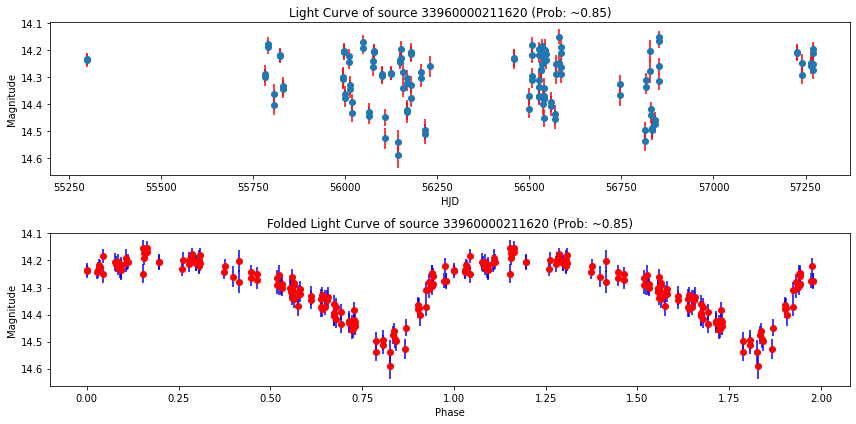
fig, axes = plt.subplots(2, 1, figsize=(12, 6))

ax = axes[0]
ax.errorbar(time, mag, err, ls="", marker="o", ecolor="red")
ax.set_title(f"Light Curve of source {rr.id} (Prob: ~{rr.prob:.2f})")
ax.set_ylabel("Magnitude")
ax.set_xlabel("HJD")
ax.invert_yaxis()

ax = axes[1]
ax.errorbar(phases, pmag, perr, ls="", marker="o", ecolor="blue", color="red")
ax.set_title(f"Folded Light Curve of source {rr.id} (Prob: ~{rr.prob:.2f})")
ax.set_ylabel("Magnitude")
ax.set_xlabel("Phase")
ax.invert_yaxis()

fig.tight_layout()

import datetime as dt
dt.datetime.now()

datetime.datetime(2022, 6, 13, 0, 25, 59, 228809)