Light-Curves catalogs tutorial (lc)

This notebook give some insights about the data stored in all the lc types catalogs.

# import the module and instance the client
import carpyncho
client = carpyncho.Carpyncho()

df = client.get_catalog("b214", "lc")
df.sample(3)

b214-lc: 222MB [01:33, 2.37MB/s]

	bm_src_id	pwp_id	pwp_stack_src_id	pwp_stack_src_hjd	pwp_stack_src_mag3	pwp_stack_src_mag_err3
10436285	32140000106633	4707	3000470700094773	56110.056177	15.774	0.053
17718411	32140000156103	4719	3000471900157271	55435.200210	17.899	0.277
20185341	32140000399685	4726	3000472600347001	56214.078852	16.240	0.073

The columns of this catalog are

print(list(df.columns))

['bm_src_id', 'pwp_id', 'pwp_stack_src_id', 'pwp_stack_src_hjd', 'pwp_stack_src_mag3', 'pwp_stack_src_mag_err3']

Where

• bm_src_id (Band-Merge Source ID): This is the unique identifier of every light curve. The records with the same bm_src_id are part of the same lc (This id is part of Carpyncho internal and is unique for every source).
• pwp_id (Pawprint Stack ID): The id of the pawprint where this point of the light curve is located (This id is part of Carpyncho internal database).
• pwp_stack_src_id (Pawprint Stack Source ID): The id of this particular observation inside the pawprint where this point (This id are part of Carpyncho internal database)
• pwp_stack_src_hjd (Pawprint Stack Source HJD): The Heliocentric-Julian-Date of this particular observation.
• pwp_stack_src_mag3 (Pawprint Stack Source Magnitude of the 3rd Aperture): The magnitude (of the 3rd aperture) of this particular observation.
• pwp_stack_src_mag_err3 (Pawprint Stack Source Magnitude Error of the 3rd Aperture): The magnitude error (of the 3rd aperture) of this particular observation.

Retrieve a single light-curve

Lets, for example, retrieve the LC with the ID 32140000349109 and sort by time

lc = df[df.bm_src_id == 32140000349109]
lc = lc.sort_values("pwp_stack_src_hjd")
lc

	bm_src_id	pwp_id	pwp_stack_src_id	pwp_stack_src_hjd	pwp_stack_src_mag3	pwp_stack_src_mag_err3
9824315	32140000349109	4705	3000470500316153	55301.355623	15.736	0.045
15823573	32140000349109	4713	3000471300371137	55404.204420	15.705	0.040
17889825	32140000349109	4719	3000471900344310	55435.200224	15.734	0.042
15383198	32140000349109	4711	3000471100264253	55497.035605	15.868	0.061
7230797	32140000349109	4694	3000469400252478	55806.201062	15.795	0.060
...	...	...	...	...	...	...
17498325	32140000349109	4718	3000471800253351	57248.183650	15.750	0.050
20689532	32140000349109	4728	3000472800102886	57251.230468	15.828	0.099
7873271	32140000349109	4697	3000469700250665	57252.177815	15.727	0.050
12365892	32140000349109	4677	3000467700294240	57265.086562	15.773	0.055
15027768	32140000349109	4686	3000468600357522	57282.060899	15.748	0.045

67 rows × 6 columns

Great, 67 epochs. Let’s check the average and dispersion of the magnitudes and the error

lc[['pwp_stack_src_mag3', 'pwp_stack_src_mag_err3']].mean()

pwp_stack_src_mag3        15.759224
pwp_stack_src_mag_err3     0.051299
dtype: float64

lc[['pwp_stack_src_mag3', 'pwp_stack_src_mag_err3']].std()

pwp_stack_src_mag3        0.044732
pwp_stack_src_mag_err3    0.009130
dtype: float64

The source is stable, now check the observation range

print((lc.pwp_stack_src_hjd.max() - lc.pwp_stack_src_hjd.min()) / 365, "Years")

5.426589796388058 Years

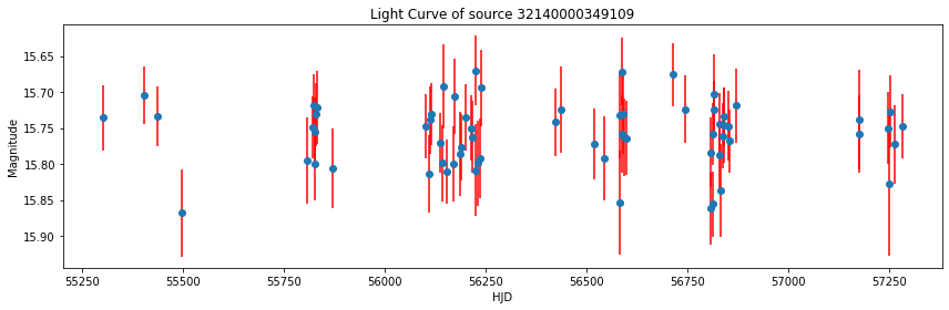
Finally we can plot the entire LC

import matplotlib.pyplot as plt

fig, ax = plt.subplots(figsize=(12, 4))

ax.errorbar(
    lc.pwp_stack_src_hjd,
    lc.pwp_stack_src_mag3,
    lc.pwp_stack_src_mag_err3,
    ls="", marker="o", ecolor="red")

ax.set_title(f"Light Curve of source 32140000349109")
ax.set_ylabel("Magnitude")
ax.set_xlabel("HJD")

ax.invert_yaxis()
fig.tight_layout()

import datetime as dt
dt.datetime.now()

datetime.datetime(2022, 6, 13, 0, 7, 52, 200684)