Features catalogs tutorial (features)

This notebook give some insights about the data stored in all the features types catalogs.

# import the module and instance the client
import carpyncho
client = carpyncho.Carpyncho()

Now we download one features catalog

df = client.get_catalog("b214", "features")
df.sample(3)

b214-features: 159MB [01:06, 2.40MB/s]

	id	cnt	ra_k	dec_k	vs_type	vs_catalog	Amplitude	Autocor_length	Beyond1Std	Con	...	c89_jk_color	c89_m2	c89_m4	n09_c3	n09_hk_color	n09_jh_color	n09_jk_color	n09_m2	n09_m4	ppmb
246230	32140000304888	66	281.886621	-24.814519			0.18675	1.0	0.287879	0.0	...	0.790576	15.292760	15.256852	0.274868	0.188890	0.602440	0.791330	15.479110	15.486869	2.341868
375156	32140000459091	44	281.626075	-24.136333			0.27050	1.0	0.431818	0.0	...	0.475020	16.945470	16.877186	0.682651	-0.076031	0.551810	0.475779	17.051519	17.072001	4.627671
264628	32140000328959	39	281.817479	-24.701575			0.28200	1.0	0.333333	0.0	...	0.498984	16.798042	16.762198	0.305437	0.071062	0.428715	0.499777	16.923741	16.932339	0.928964

3 rows × 73 columns

The columns of this catalog are

print(list(df.columns))

['id', 'cnt', 'ra_k', 'dec_k', 'vs_type', 'vs_catalog', 'Amplitude', 'Autocor_length', 'Beyond1Std', 'Con', 'Eta_e', 'FluxPercentileRatioMid20', 'FluxPercentileRatioMid35', 'FluxPercentileRatioMid50', 'FluxPercentileRatioMid65', 'FluxPercentileRatioMid80', 'Freq1_harmonics_amplitude_0', 'Freq1_harmonics_amplitude_1', 'Freq1_harmonics_amplitude_2', 'Freq1_harmonics_amplitude_3', 'Freq1_harmonics_rel_phase_0', 'Freq1_harmonics_rel_phase_1', 'Freq1_harmonics_rel_phase_2', 'Freq1_harmonics_rel_phase_3', 'Freq2_harmonics_amplitude_0', 'Freq2_harmonics_amplitude_1', 'Freq2_harmonics_amplitude_2', 'Freq2_harmonics_amplitude_3', 'Freq2_harmonics_rel_phase_0', 'Freq2_harmonics_rel_phase_1', 'Freq2_harmonics_rel_phase_2', 'Freq2_harmonics_rel_phase_3', 'Freq3_harmonics_amplitude_0', 'Freq3_harmonics_amplitude_1', 'Freq3_harmonics_amplitude_2', 'Freq3_harmonics_amplitude_3', 'Freq3_harmonics_rel_phase_0', 'Freq3_harmonics_rel_phase_1', 'Freq3_harmonics_rel_phase_2', 'Freq3_harmonics_rel_phase_3', 'Gskew', 'LinearTrend', 'MaxSlope', 'Mean', 'Meanvariance', 'MedianAbsDev', 'MedianBRP', 'PairSlopeTrend', 'PercentAmplitude', 'PercentDifferenceFluxPercentile', 'PeriodLS', 'Period_fit', 'Psi_CS', 'Psi_eta', 'Q31', 'Rcs', 'Skew', 'SmallKurtosis', 'Std', 'StetsonK', 'c89_c3', 'c89_hk_color', 'c89_jh_color', 'c89_jk_color', 'c89_m2', 'c89_m4', 'n09_c3', 'n09_hk_color', 'n09_jh_color', 'n09_jk_color', 'n09_m2', 'n09_m4', 'ppmb']

Where

• id (ID): This is the unique identifier of every light curve. If you want to access all the points of the lightcurve of a source wiht any id, you can search for the same value of a bm_src_idin the lc of the same tile of the features catalog.
• cnt (Count): How many epochs has the lightcurve.
• ra_k: Right Ascension in band \(K_s\) of the source in the first epoch.
• dec_k: Declination in band \(K_s\) of the source in the first epoch.
• vs_type (Variable Star Type): The type of the source if is a variable star tagged with the OGLE-III, OGLE-IV and VIZIER catalogs; or empty if the source has no type.
• vs_catalog (Variable Star Catalog): From which catalog the vs_type was extracted.

All the other columns (Except the last 13) are the features itself And can be consulted here https://feets.readthedocs.io/en/latest/tutorial.html#The-Features

Finally the reddening free features are:

• c89_c3: \(C3\) Pseudo-color using the cardelli-89 extinction law.

• c89_ab_color: Magnitude difference in the first epoch between the band \(a\) and the band \(b\) using the Cardelli-89 extinction law. Where \(a\) and \(b\) can be the bands \(H\), \(J\) and \(K_s\).

• c89_m2 and c89_m4: \(m2\) and \(m4\) pseudo-magnitudes using the Cardelli-89 extinction law.

• n09_c3: \(C3\) Pseudo-color using the Nishiyama-09 extinction law.

• n09_ab_color: Magnitude difference in the first epoch between the band \(a\) and the band \(b\) using the nishiyama-09 extinction law. Where \(a\) and \(b\) can be the bands \(H\), \(J\) and \(K_s\)

• n09_m2 and n09_m4: \(m2\) and \(m4\) pseudo-magnitudes using the nishiyama-09 extinction law.

• ppmb (Pseudo-Phase Multi-Band): This index sets the first time in phase with respect to the average time in all bands, using the period calculated by feets.

  \[PPMB = frac(\frac{|mean(HJD_H, HJD_J, HJD_{K_s}) - T_0|}{P})\]

  Where \(HJD_H\), \(HJD_J\) and \(HJD_{K_s}\) are the time of observations in the band \(H\), \(J\) and \(K_s\); \(T_0\) is the time of observation of maximum magnitude in \(K_s\) band; \(mean\) calculate the mean of the three times, \(frac\) returns only the decimal part of the number, and \(P\) is the extracted period.

For more information about the extintion laws and pseudo colors/magnitudes:

---

Cardelli-89 Extinction law:

Cardelli, J. A., Clayton, G. C., & Mathis, J. S. (1989). The relationship between infrared, optical, and ultraviolet extinction. The Astrophysical Journal, 345, 245-256.

Nishiyama-09 Extinction law:

Nishiyama, S., Tamura, M., Hatano, H., Kato, D., Tanabé, T., Sugitani, K., & Nagata, T. (2009). Interstellar extinction law toward the galactic center III: J, H, KS bands in the 2MASS and the MKO systems, and 3.6, 4.5, 5.8, 8.0 μm in the Spitzer/IRAC system. The Astrophysical Journal, 696(2), 1407.

Pseudo colors/magnitudes:

Catelan, M., Minniti, D., Lucas, P. W., Alonso-Garcia, J., Angeloni, R., Beamin, J. C., … & Dekany, I. (2011). The Vista Variables in the Via Lactea (VVV) ESO Public Survey: Current Status and First Results. arXiv preprint arXiv:1105.1119.

Well lets play with the data of 3 Variable star

rrs = df[df.vs_type == "RRLyr-RRab"][:3]
rrs

	id	cnt	ra_k	dec_k	vs_type	vs_catalog	Amplitude	Autocor_length	Beyond1Std	Con	...	c89_jk_color	c89_m2	c89_m4	n09_c3	n09_hk_color	n09_jh_color	n09_jk_color	n09_m2	n09_m4	ppmb
4456	32140000002913	68	280.582129	-25.299033	RRLyr-RRab	vizier	0.12600	1.0	0.279412	0.0	...	0.162897	13.827993	13.819663	0.053522	0.040231	0.123061	0.163291	13.893530	13.895081	1.629816
21827	32140000030432	68	280.482488	-25.156328	RRLyr-RRab	vizier	0.17275	1.0	0.235294	0.0	...	0.221322	13.112390	13.104045	0.049464	0.062893	0.158674	0.221566	13.185733	13.187114	1.672651
21929	32140000030564	68	281.279492	-25.499744	RRLyr-RRab	vizier	0.18400	1.0	0.308824	0.0	...	0.314535	14.001622	13.984766	0.128221	0.068086	0.246717	0.314803	14.087323	14.090839	2.006219

3 rows × 73 columns

We can check their mean of magnitudes to check if the source is not saturated or diffuse.

rrs.Mean

4456     14.086691
21827    13.488265
21929    14.412221
Name: Mean, dtype: float64

The three are between 12 an 16.5, so they are ok, and their pulsation?

rrs.Std

4456     0.071391
21827    0.090222
21929    0.120290
Name: Std, dtype: float64

Plotting time: we need the lc catalog to show the phased-folded light curve.

lcs = client.get_catalog("b214", "lc")

Now to reduce the memory footprint we can retrieve the lc for only our 3 selected stars

lcs = lcs[lcs.bm_src_id.isin(rrs.id)]

For make our code simple we can use to folde the light curve the PyAstronomy and numpy library

from PyAstronomy.pyasl import foldAt
import numpy as np

%matplotlib inline
import matplotlib.pyplot as plt

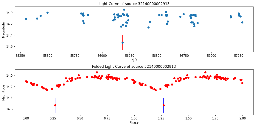
now we can plot the folded and unfolded lightcurves

# get one ot the 3 sources
rr = rrs.iloc[0]

# retrieve the lightcurve for this rr
lc = lcs[lcs.bm_src_id == rr.id]

# sort by time
lc = lc.sort_values("pwp_stack_src_hjd")

# split in time, magnitude and error
time, mag, err = (
        lc.pwp_stack_src_hjd.values,
        lc.pwp_stack_src_mag3.values,
        lc.pwp_stack_src_mag_err3.values)

# t0 is the first time
t0 = time[0]

# fold
phases = foldAt(time, rr.PeriodLS, T0=t0)
sort = np.argsort(phases)
phases, pmag, perr = phases[sort], mag[sort], err[sort]

# duplicate the values in two phases
phases = np.hstack((phases, phases + 1))
pmag = np.hstack((pmag, pmag))
perr = np.hstack((perr, perr))

# now create two plot for the folded and the unfolde LC
fig, axes = plt.subplots(2, 1, figsize=(12, 6))

# first lets plot the unfolded lc
ax = axes[0]
ax.errorbar(time, mag, err, ls="", marker="o", ecolor="red")
ax.set_title(f"Light Curve of source {rr.id}")
ax.set_ylabel("Magnitude")
ax.set_xlabel("HJD")
ax.invert_yaxis()

# now the folded lc
ax = axes[1]
ax.errorbar(phases, pmag, perr, ls="", marker="o", ecolor="blue", color="red")
ax.set_title(f"Folded Light Curve of source {rr.id}")
ax.set_ylabel("Magnitude")
ax.set_xlabel("Phase")
ax.invert_yaxis()

fig.tight_layout()

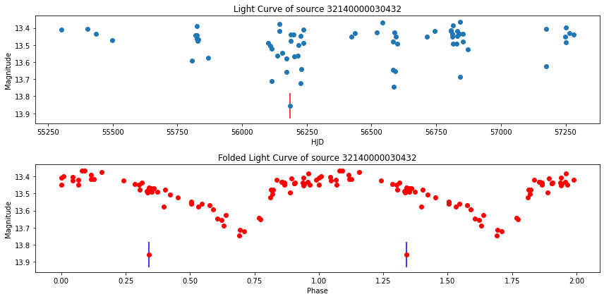
The next light curve

rr = rrs.iloc[1]
lc = lcs[lcs.bm_src_id == rr.id]
lc = lc.sort_values("pwp_stack_src_hjd")

time, mag, err = (
        lc.pwp_stack_src_hjd.values,
        lc.pwp_stack_src_mag3.values,
        lc.pwp_stack_src_mag_err3.values)

t0 = time[0]

phases = foldAt(time, rr.PeriodLS, T0=t0)
sort = np.argsort(phases)
phases, pmag, perr = phases[sort], mag[sort], err[sort]

phases = np.hstack((phases, phases + 1))
pmag = np.hstack((pmag, pmag))
perr = np.hstack((perr, perr))


fig, axes = plt.subplots(2, 1, figsize=(12, 6))

ax = axes[0]
ax.errorbar(time, mag, err, ls="", marker="o", ecolor="red")
ax.set_title(f"Light Curve of source {rr.id}")
ax.set_ylabel("Magnitude")
ax.set_xlabel("HJD")
ax.invert_yaxis()

ax = axes[1]
ax.errorbar(phases, pmag, perr, ls="", marker="o", ecolor="blue", color="red")
ax.set_title(f"Folded Light Curve of source {rr.id}")
ax.set_ylabel("Magnitude")
ax.set_xlabel("Phase")
ax.invert_yaxis()

fig.tight_layout()

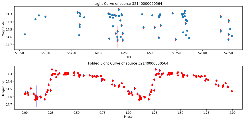
And the final one

rr = rrs.iloc[2]
lc = lcs[lcs.bm_src_id == rr.id]
lc = lc.sort_values("pwp_stack_src_hjd")

time, mag, err = (
        lc.pwp_stack_src_hjd.values,
        lc.pwp_stack_src_mag3.values,
        lc.pwp_stack_src_mag_err3.values)

t0 = time[0]

phases = foldAt(time, rr.PeriodLS, T0=t0)
sort = np.argsort(phases)
phases, pmag, perr = phases[sort], mag[sort], err[sort]

phases = np.hstack((phases, phases + 1))
pmag = np.hstack((pmag, pmag))
perr = np.hstack((perr, perr))


fig, axes = plt.subplots(2, 1, figsize=(12, 6))

ax = axes[0]
ax.errorbar(time, mag, err, ls="", marker="o", ecolor="red")
ax.set_title(f"Light Curve of source {rr.id}")
ax.set_ylabel("Magnitude")
ax.set_xlabel("HJD")
ax.invert_yaxis()

ax = axes[1]
ax.errorbar(phases, pmag, perr, ls="", marker="o", ecolor="blue", color="red")
ax.set_title(f"Folded Light Curve of source {rr.id}")
ax.set_ylabel("Magnitude")
ax.set_xlabel("Phase")
ax.invert_yaxis()

fig.tight_layout()

import datetime as dt
dt.datetime.now()

datetime.datetime(2022, 6, 13, 0, 13, 25, 563015)